The program implements a variety of established techniques, most of which are reviewed in the following paper about hybrid modeling methods:

Willy Wriggers and Pablo Chacón. Modeling Tricks and Fitting Techniques for Multi-Resolution Structures. Structure, 2001, Vol. 9, pp. 779-788. [Article]

The efficient feature-based M-to-N docking algorithm is described in the following article:

Stefan Birmanns and Willy Wriggers. Multi-Resolution Anchor-Point Registration of Biomolecular Assemblies and Their Components. J. Struct. Biol. 2007, Vol. 157, pp. 271-280. [Article]

The user manual describes the individual menu-items one by one - the tutorial section reports in a more application oriented fashion how one can carry out a multi-resolution fitting.

Set Target Map

- As one can load multiple data sets into Sculptor, the user has to inform the program which of the files is the target map for the multi-resolution fitting. Once the document is selected, a small icon next to its file-name will also show its special state as target map:

The volumetric map which was loaded last will automatically be selected as target map.

Set Probe Molecule

- As one can load multiple data sets into Sculptor, the user has to inform the program which of the files is the probe-molecule for the multi-resolution fitting.

The structure which was loaded last will automatically be selected as probe molecule.

Cross Correlation

- In signal processing cross-correlation is an established criterion to determine the agreement or similarity of two signals. It can be used in the context of multi-resolution fitting as scoring function to compare multiple docking solutions.

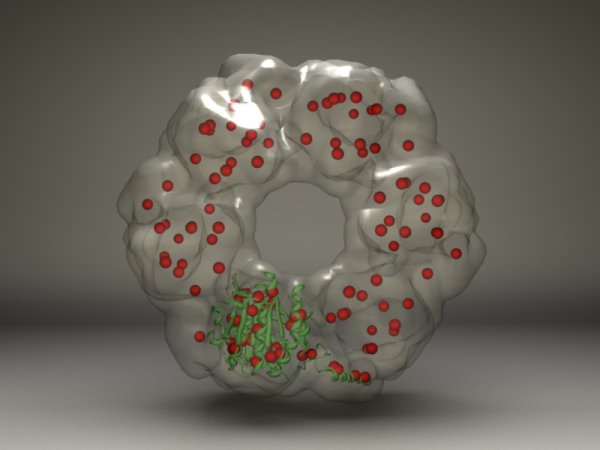
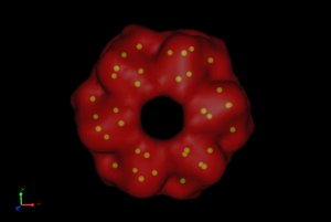
Select two volumetric maps from the list of documents and click on the cross-correlation menu item. The program will calculate and report the cross-correlation coefficient between the two maps. If a structure was docked into a map and the quality of the fit should be measured using the CCC, the structure has to be converted into a volumetric description first. Please click on the document and selected "Structure->Blur" to generate a volumetric map. The resulting volume can then be utilized in a second step for the correlation coefficient calculation.

Feature Extraction

The items in the sub-menu extract feature-points from multi-resolution data sets. These feature-points can then in a second step be utilized to find solutions to the multi-resolution docking problem (see feature-based docking below).

Feature-points can be determined using the neural gas algorithm or laplacian quantization. The algorithmic details are described in the following article:

Stefan Birmanns and Willy Wriggers. Multi-Resolution Anchor-Point Registration of Biomolecular Assemblies and Their Components. J. Struct. Biol. 2007, Vol. 157, pp. 271-280. [Article]

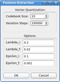
Neural Gas:

The neural gas is a classic artificial neural network algorithm, from the category of the self-organizing maps. The neural net is trained to represent the original data in a best possible way (least information loss). After clicking on "Feature Extraction->Neural Gas" the following dialog box appears:

The main parameter is the size of the codebook, which determines the number of the features the algorithm will extract from the data. The other parameters concern the inner workings of the algorithm, they should not be changed in common docking applications. The following article describes the algorithm and the parameters:

A "neural-gas" network learns topologies. In T. Kohonen, K. Mäkisara, O. Simula, and J. Kangas, editors, Artificial Neural Networks, pages 397-402. North-Holland, Amsterdam, 1991.

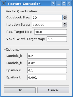
Laplacian Quantization:

The laplacian quantization combines the laplacian filter with the vector quantization algorithm, yielding in superior performance for volumetric maps with a low resolution. In order to be able to apply the laplace filter the algorithm will convert the high-resolution structures into volumetric maps internally. In order to be consistent, the algorithm needs to know the resolution and voxel width of the target map when quantizing a structure:

Atomic Coordinates:

This option is typically not useful for a normal multi-resolution docking application - it provides a simple feature extraction based on the atomic coordinates of a molecular structure. This is only useful for the comparison of two structures, do not use this option and compare the feature vectors with neural gas generated points!

Import / Export Feature Vectors:

The feature vectors are stored by default in the Sculptor state file ("File->Save State" and "File->Load State", see the documentation of the File menu). If one would like to use already previously calculated feature-points from another program (for example from the Situs qpdb and qvol tools), or if one would like to export the coordinates to other programs, one can use Sculptor to import or export the points in PDB format.

Render Feature Vectors

The visualization of the feature vectors can be turned on or off with this menu item:

Render Displacements

In addition to the normal feature-vector rendering one can also render the deviation of two feature-point sets using arrows (for example in order to visualize the conformational change between two data sets). Please select two documents in the document list (hold down the ctrl key and click onto the two documents). The two documents have to have feature-point sets associated with them (for example from a feature extraction with the neural gas algorithm). Once you click on the menu item, the visualization should change and arrows between the two point-sets will appear:

Feature-Based Docking

The menu-item represents an efficient docking technique, which utilizes feature-points to bring two data sets into register. Please see the menu-items above on how to extract those feature points from your data sets. There is also a more application-oriented step-by-step description available in the tutorial section.

The details of the efficient feature-based M-to-N docking algorithm is described in the following article:

Stefan Birmanns and Willy Wriggers. Multi-Resolution Anchor-Point Registration of Biomolecular Assemblies and Their Components. J. Struct. Biol. 2007, Vol. 157, pp. 271-280. [Article]

Before clicking on the menu-item, please make sure that the feature points were extracted from both data sets. Also make sure that both feature-point sets describe the original data with the same level of detail. In an oligomer, the whole complex has to have n-times more feature-points than the single monomer, if the complex has n subunits. In other cases one can also use the molecular mass, number of atoms or other physical entities to ensure that the number of feature points is consistent in both data sets.

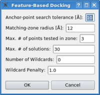
Please select the target map and the probe molecule using the "Docking->Set Target Map", "Docking->Set Probe Molecule" menu-items. Now click on the "Docking->Feature-Based Docking" item. The following dialog-box will appear:

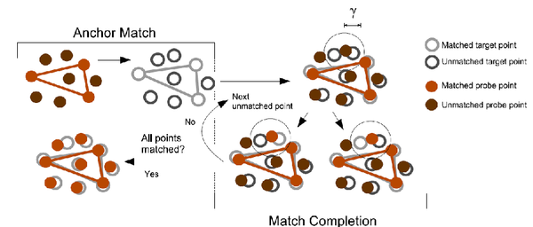
The parameters reflect the pruning of the hierarchical matching, please see article for details. As a rule of thumb, if there are no or not enough solutions, increase the parameters from top to bottom in the dialog box, in order to increase the thresholds of the search. See following schema for a brief summary of how the algorithm finds the solutions:

The first parameter in the dialog box reflects the tolerance in the first stage of the search (anchor match) - the higher the value, the more potential solutions are found. Increase the parameter slowly, the run-time might increase dramatically. The second parameter specifies the size of the search area in the match completion phase. Increase this parameter also very carefully and only after increasing the first parameter did result in a higher number of potential solutions, but not in enough final solutions. The maximum number of points tested in the search zone limits the run-time - it should not be necessary to tune this parameter.

With the maximum number of solutions one can limit the output of final solutions of the algorithm. The setting also depends of the size of your complex, please allow always some more solutions than you have subunits in your system.

The number of wildcards can be increased in case of noticeable deviations between the feature-point sets. The feature-points might fluctuate more in case of low-resolution maps, in case of conformational differences or artifacts in the volumetric data. In those cases the algorithm can be forced to be tolerant and accept solutions even if not all feature-points can be mapped successfully. The resulting partially matched point sets render a correct ranking difficult - is a solution with a higher rmsd but complete matching favorable over a solution with a lower rmsd but some unmatched points? The ranking can be influenced by adjusting the wildcard penalty - if increased the solutions with unmatched points are penalized and typically will rank lower.

Refinement

Already docked solutions can be refined using correlation-based scoring functions. Please see the tutorial section for details.

Transformation

In multi-scale modeling applications a precise control over the transformations applied to the probe molecule is necessary to ensure an accurate docking result. Therefore Sculptor provides two basic modes of interactions: With the mouse molecular structures can be moved on the X-Y plane (right mouse button), on the X-Z plane (middle mouse button) and rotate around the origin (left mouse button).

- if precise control is needed, a transformation dialog can be activated (menu: 'Docking->Transformation').

Six dials control the six degrees of freedom of a transformation in 3D space. The top dials determine the three translation components, a translation along the X, the Y, and the Z axis. Each step on one of the dials corresponds to 0.1 Angstroem.
The lower three dials determine the three components of the rotation, along the X, the Y, and the Z axis. Each step rotates the object by 1 degree