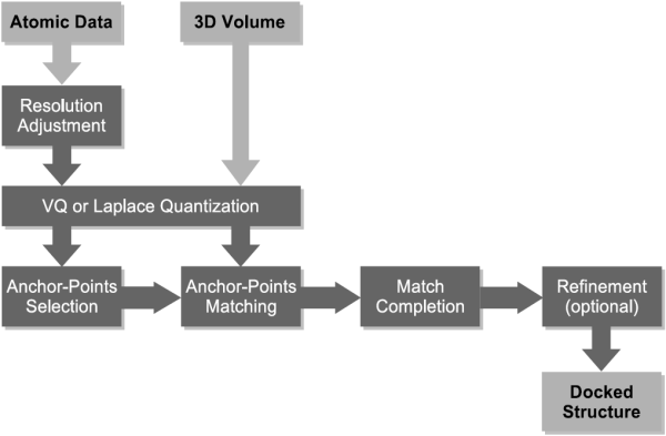
In the following our "classic" solution to the multi-resolution docking problem is described. Multi-resolution docking describes the task of fitting high-resolution atomic structures into low-resolution volumetric maps. The low-resolution maps are most often the result of single-particle cryo-EM reconstructions, but also tomographic reconstructions and even SAXS bead models were successfully interpreted using the technique described in this document.

Feature-based docking utilizes vector quantization to perform a dimensionality reduction of the multi-resolution data sets. Vector quantization is a method from signal processing and is used here to determine feature-points that encode the low-resolution volumetric data as well as the high-resolution atomic structure. This way, both types of data are brought to a comparable level of detail, which ensures a robust and stable behavior in the presence of artifacts and noise in the experimental data. Both feature-point sets are then used to perform a pattern matching procedure, which finds similar subsets of points and delivers thereby a solution to the multi-resolution docking problem.

The following schema gives an overview over the entire work-flow:

Data Sets

In a first step the data sets have to be loaded into Sculptor - please download the following files (right-click, "Save Link As"):

1. 2rec15.situs
   (volumetric map of the reca hexamer - 15A resolution)
2. 2recmon.pdb
   (atomic structure of the monomer)
3. 2REC.pdb
   (atomic coordinates of the full hexamer, for validation only)

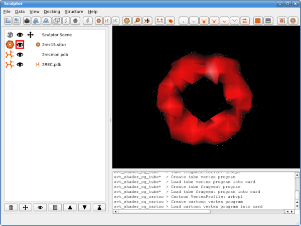
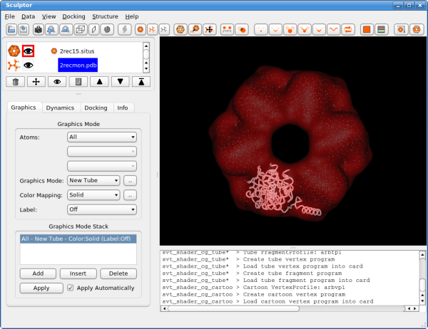
The atomic data can then be convolved with a Gaussian kernel to bring the resolution to a similar level as found in the volumetric data. This step is optional as the vector quantization procedure adjusts the level of detail anyway and as the correct resolution of a volumetric map is not trivial to determine.

After downloading the data, please open them using the "file->open" menu-item. Hint: One can select multiple files in the file-open dialog and thereby load all three files at the same time.

You should see now the three documents being listed in the top-left part of the main graphical user interface. Please adjust the order of the documents so that 2rec15.situs is the first document in the list - use the up and down arrows to reorder the entries if necessary.

Your Sculptor window should now look like this:

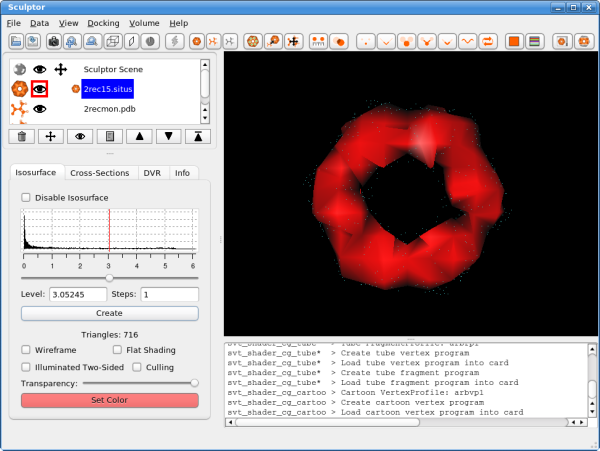
Visualization

The visualization performed here is rather basic and does not show all the capabilities of Sculptor - please refer to the other documentation to get a more complete overview of the visualization features of Sculptor.

Please start by clicking on the 2rec15.situs document. Now the main volume-rendering dialog appears right below the document list.

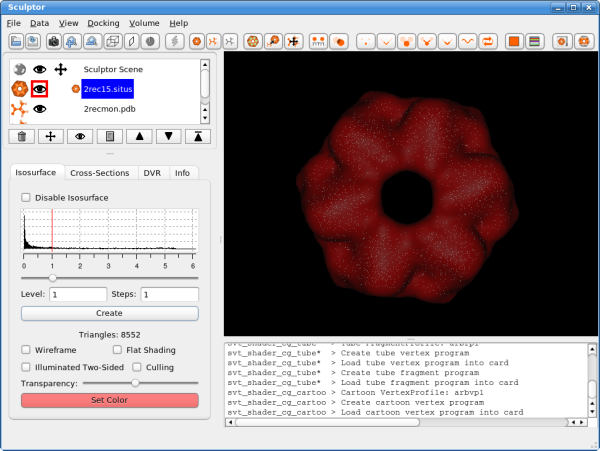
Click into the histogram to change the iso-surface threshold value. Adjust it to 1.0 (alternatively the level can also be typed in numerically - enter or clicking on the "Create" button will update the rendering). As the atomic structure needs to be docked into the volume, we have to render the low-resolution data in a transparent or semi-transparent way. This can be accomplished by either using the "Transparency" slider - moving it to the left makes the volume data more transparent. Another possibility is the "wireframe" mode.

Now click on the next document in the list, the atomic structure of the monomer: 2recmon.pdb. The part just below the document list changes and shows now the rendering options for the atomic structures. Please select the "Graphics Mode" pull-down menu and select "New Tube". Please adjust also the color of the rendering by clicking on "Color Mapping" and setting it to "Solid". Now click on the button with the dots right next to "Color Mapping: Solid" field. A new color selector dialog is shown now and please select a bright color for the probe structure.

You window should now look like the following:

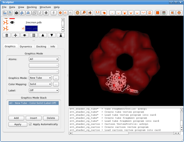
Please click now also on the last document in the list, the structure of the entire hexamer "2REC.pdb", and adjust the rendering to "New Tube" and select a different color.

As the "2REC.pdb" is only used for validation, we can now make it invisible by clicking on the eye symbol in the document list. The eye icon and the rendering of the hexameric structure should disappear.

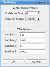
Feature Extraction

As the documents are now loaded and properly visualized, we can now move on and determine the feature-points. Select the probe structure "2recmon.pdb" in the document list. Now click into the "Docking" menu and select the "Feature-Extraction" submenu and click on the first menu-item: "Neural Gas":

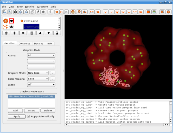
Select 6 for "codebook size" (number of feature-points) and click on "OK" to start the calculation. Briefly a progress bar should appear on the bottom part of the main window, but even on a low-end PC the calculation should not take longer than a few seconds.

The resulting feature vectors are shown as spheres in the 3D window:

Now click also on the first document "2rec15.situs" and calculate the feature points by selecting "Docking"->"Feature Extraction"->"Neural Gas". As there are 6 monomers in the system, please choose a codebook size of 36 and click on "OK". As the codebook is larger compared to the other data set, the calculation will be longer this time, but should again finish in less than one minute.

As we have loaded multiple structures, we now have to select the correct probe molecule we would like to dock into the volume. Therefore, please select "2recmon.pdb" in the document list and click on "Docking"->"Set Probe Molecule". Now a little orange structure symbol should appear in the document list entry, immediately left of the filename.

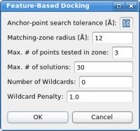
Automatic Docking

The two feature point sets - represented by the red and green spheres in the 3D window - are now being used to dock the structure. Please click on "Docking"->"Feature-Based Docking" - the following dialog box should appear now:

For the tutorial here, no changes in the parameters are necessary. If the parameters do not work in the case of your own system, please adjust the values in the following order:

1. If you do not get any solutions at all, increase the anchor-point search tolerance. Using higher values will let the algorithm find more anchor-point triangles. Increase the values in small steps as high-values can lead to excessive run-times as too many anchor-point triangles have to be considered.
2. If you still do not get any solutions at all try to increase the number of wildcards. Depending on the total number of codebook vectors, one should select between 1 and 3 wildcards. Only very large systems might require more. Wildcards are very useful if individual codebook vectors are unstable, for example because of different resolutions throughout the volumetric map or other artifacts.
3. Increase the matching zone radius. Again, increase the value slowly to avoid very long run-times.

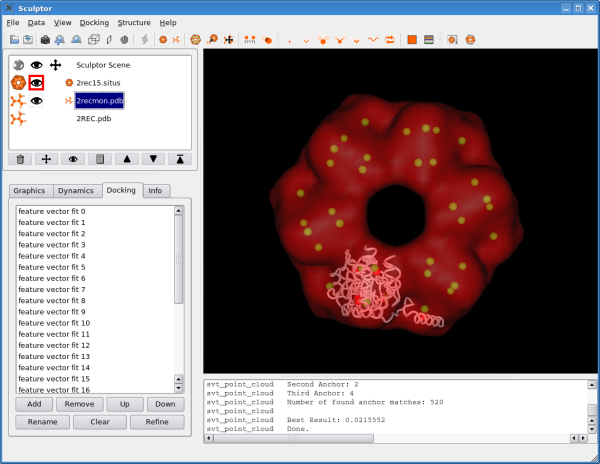
Clicking on "OK" will start the pattern-matching algorithm. The matching should finish within a few seconds and a list of all found solutions is presented, sorted based on the docking score:

Inspection of the Results

Double-clicking on a solution in the list will transform the probe-molecule immediately to the appropriate position and orientation. Double-clicking on the first solutions in the list will show you the correctly docked monomers of the RecA hexamer. In this test case, we also have the complete atomic structure of all monomers available and can actually check the validity of the docking results. Therefore please click now on the last document "2REC.pdb" in the document list. Now click on the left, into the area where there was the eye with which one can toggle the visibility of the document. The eye-icon and the 3D rendering of the structure should re-appear now. You should see that the docked structure represents one of the monomers, although there is some deviation from the correct solution.

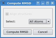
In the document list one can actually select multiple items by pressing the "crtl" key on the keyboard and clicking onto the documents one wishes to select. Please select now the docked monomer "2recmon.pdb" and the hexamer "2REC.pdb" - both should get a blue background. Now do a right click onto "2recmon.pdb" and click on "RMSD". Do not change any option in the dialog box and just click on "calculate rmsd". This function measures the rms deviation between the docked monomer and the correct solution - it should be in a 1-2 Angstroem range. The slight fluctuation of the docking results depends on the resoution of the volumetric map - which is comparatively low in the case here.

Storing and Exporting the Docked Structures

We recommend to inspect the docking results thoroughly - obviously misplaced structures should be deleted from the solution list, top solutions can be renamed to be recognized more easily, etc. As this inspection phase might take some time, one can save the entire state of Sculptor into a file. These Sculptor scene files will store the information about all visualization settings, but also the information about the docking solutions. The individual solutions will only get stored as transformations, the atomic coordinates are not getting duplicated - this way also long lists of potential docking solutions can be stored efficiently. To store our results so far, click on "File"->"Save State" and save the current docking to a ".scl" file with a name of your choice. If the file was written to disk successfully, one can quite Sculptor safely and load the same docking results back in, later.

Warning: The Sculptor state file will save all settings, information about the visualization and the docking results, but it will not store the data from your volume file or the pdb file internally! It will only store the filenames, if you move the data files to another directory or delete them, the state file is invalid and Sculptor will not be able to restore the docking situation later.

At some point the multi-resolution docking of the system is finished and one typically wishes to export the pdb files of the docked monomers. Double click on the particular solution in the solution list and then click on "File"->"Save As". Now one can export the solution as a pdb file with the new coordinates of the docking position.

Video

The following video shows Sculptor performing the rigid-body docking described above:

Adobe Flash Player not installed or older than 9.0.115!