| Tutorial - Feature-Based Flexible Fitting |
|
Data Flow and DesignPlease note that the atomic structure and volumetric map must undergo a rigid-body alignment prior to the flexible fitting. This step is essential for the flexible fitting. Although several techniques may be utilized to perform the rigid-body registration (beyond the purpose of this tutorial), we recommend the feature-based (rigid-body) docking in Sculptor. The multi-resolution data set of RNA Polymerase provide here was already aligned.
Data setPlease download the following files (use right- click and select the "Save Link As" option):
Load DataPlease load the atomic structure from the file "rnap.pdb" and the map from "rnap.situs" using "File"->"Open" menu-item. You should now see the two documents being listed in the document list in the top-left part of the main Sculptor window. Modify the graphical representation of "rnap.pdb" to cartoon (select "rnap.pdb" in the document list to show the "Property" window, in the "Graphics" tab set "Graphics mode" to cartoon). Also, for "rnap.situs", change the color to white, decrease its transparency to ~50% and choose 2.85 as isosurface level (all options can be set from the "Property" window, "Isosurface" tab ). At this step your Sculptor window should now look like this:
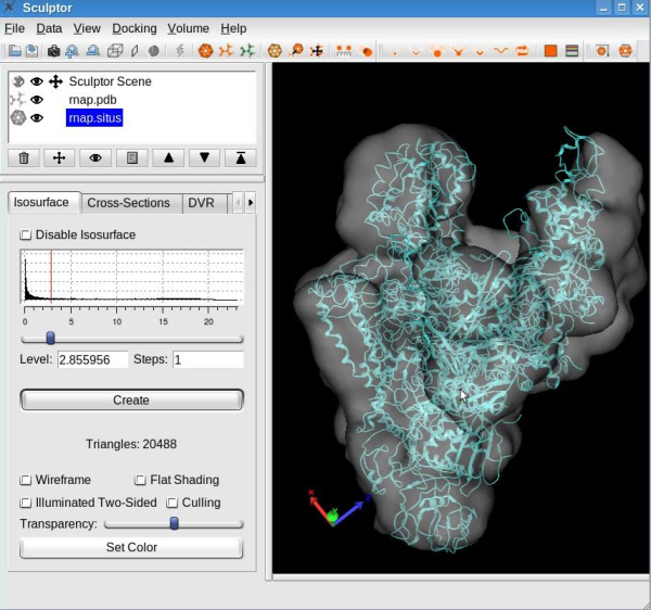
For a better view on the atomic structure, make the volumetric map invisible by clicking on the eye icon next to the volume name "rnap.situs" .
Dimensionality reduction of the atomic structureCompute the feature vectorsThe first step of flexible fitting consists of computing the feature vectors of the atomic structure. Select the atomic structure by clicking on the file name "rnap.pdb" in the document list. Use the "Docking" -> "Feature Extraction" -> "Neural gas" menu item to open the "Feature-Extraction" dialog. Set the codebook size to 15 vectors:
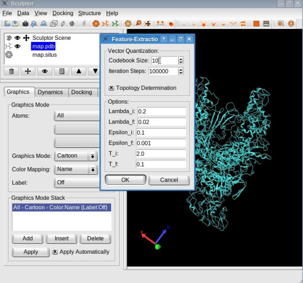
Make sure the "Topology Determination" option is checked, and then click the OK button. With the options selected, the neural gas clustering technique identifies the feature vectors as well as the connections between them. When the clustering is done, your window should look like this:
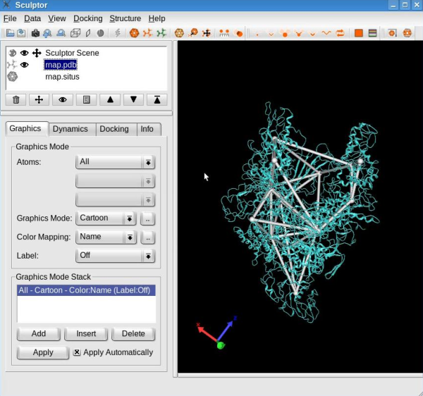
Edit the skeletonConnections between the feature vectors may be added or removed interactively. For that, first select one feature vector by holding the CTRL-key pressed and left-clicking the desired vector. The successful selection of the feature vector is indicated by its color turning yellow:
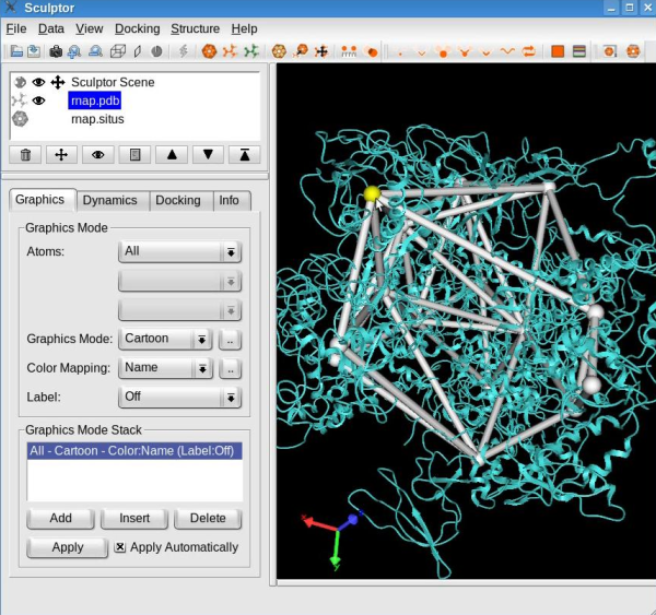
Note: To unselect a feature vector, press the right mouse button. Select a second feature vector. If a connection exists between these two selected feature vectors, this procedure will remove the connection. On the other hand, if none was present then the connection will be added.
Use this procedure to remove the connections that do not consistently overlap with the structure, in particular between the feature vectors in opposite "claws", and between "claws" and other domains (see movie below). Finish this step by making the atomic structure a probe molecule using the "Docking" -> "Set Probe Molecule" menu item.
Dimensionality reduction of the volumetric mapStart by making the volumetric map visible (press left mouse button on the eye icon next to the file name "rnap.situs"). Then select the volume by clicking the file name in the document list and make it the target map ("Docking" -> "Set Target Map"). Use the "Docking" -> "Feature Extraction" -> "Flex Feature-Vectors" menu item to open the dialog for the computation of the feature vectors of the volumetric map. This tool identifies the feature vectors of the volumetric map using the skeleton, feature vectors, and connections of the probe molecule. Leave all parameters set to default and click the OK button.
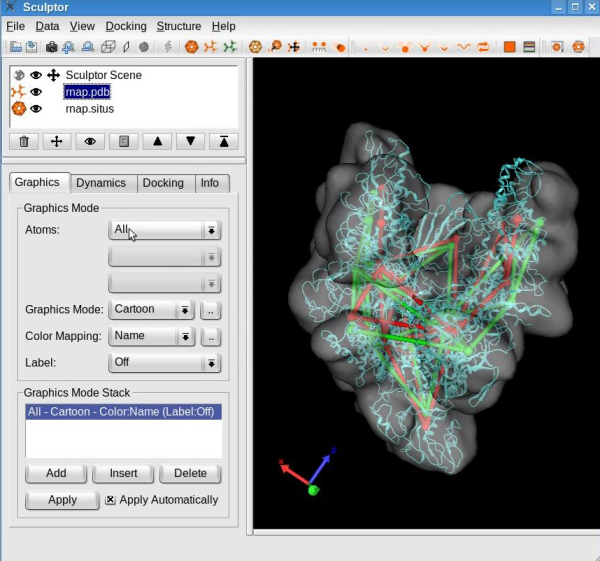
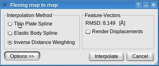
Feature-based flexing fittingNow we are set to proceed with the flexible registration. Select the "Docking" -> "Feature-Based Flexing" menu item to open the flexing dialog:
This dialog permits the selection of the flexible fitting parameters. Toggle the "Render Displacement" box to show or hide the displacement of the feature vectors between the structure and volume. Note that this dialog also shows the root mean square deviation (RMSD) measured between the feature vectors of the atomic structure and of the volumetric map. The value shown here might be different in your run.
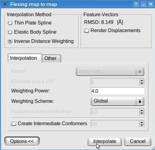
Now, click the "Options>>" button to be able to modify the default parameters of the interpolation methods. The window will look like this:
We recommend the inverse distance weighting interpolation, with the weighting power set to 4 and the global weighting scheme. Note that this window allows to select various interpolation methods and to set their parameters. Although the inverse distance weighing interpolation is recommended, other interpolation methods are available. The thin plate spline has no parameter to be set while the elastic body spline permits the selection of a kernel and the elasticity coefficient (restrained to be between 1 and 49). The values set by default represent the recommended values according to our tests (Rusu et. al., Bioinformatics 2008).
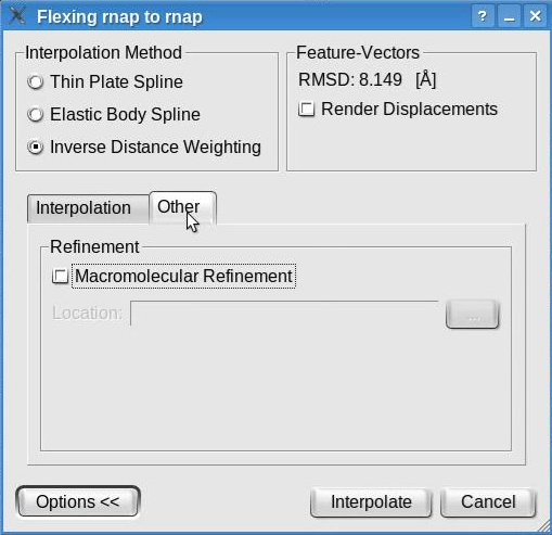
The "Other " tab displays the crystallographic refinement options:
The molecular refinement is NOT supported on Windows and may be executed only if the software tool refmac (included in the ccp4 program suite) is installed on the user's machine (not provided with Sculptor). By checking the "Molecular Refinement" box and indicating the location of the refmac executable, the structure obtained by interpolation will undergo a regularization procedure that brings bonds and angles into ideal range.
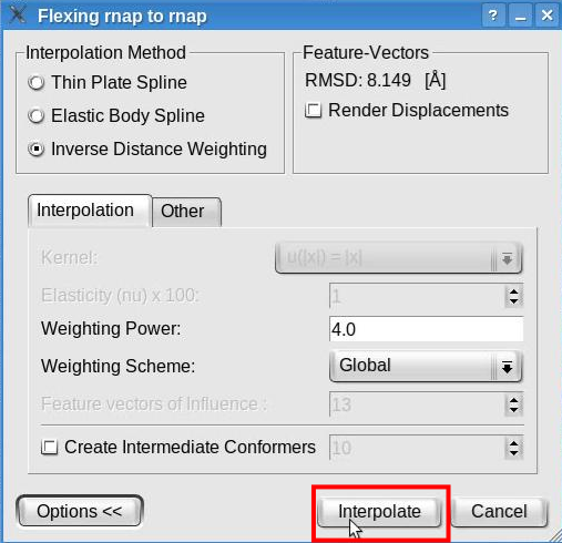
Click the "Interpolate" button to launch the interpolation:
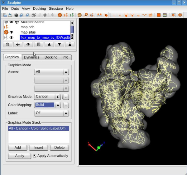
A new structure will be generated by interpolating the probe structure according to the features deviations. This structure will be added to the document list in Sculptor's main window. Please change the graphical representation of this new structure ("flex_rnap_to_rnap_by_IDW") to cartoon and hide the probe structure (in the document list, click on the eye icon left of the "rnap.pdb" ).
Your sculptor window should now look like this:
See the tutorial video:
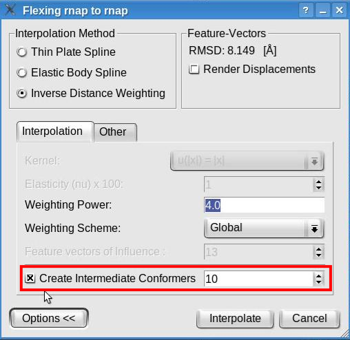
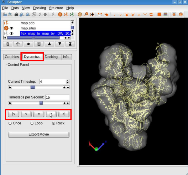
How to (better) visualize conformational differencesA simple approach to emphasize the conformational differences between the original structure and the flexed model consists in toggling the visibility of the two documents. This may be achieved by making one document visible and the other invisible (click the eye icon at left of the document name), selecting both documents (hold CTRL while left-clicking on the document names), and then clicking the eye icon below the document list to toggle the visibility of the two selected documents. Moreover, Sculptor is able to show the conformational differences of multi-resolution data sets as an animation via the interpolation method. The interpolation allows for intermediate conformers to be created between the original and the flexed structure. These intermediate conformers can be shown in an animation, thereby demonstrating the conformational differences between data sets. Launch the flexible fitting from the "Docking" -> "Feature Based Flexing" menu item. In the expanded options of the flexing dialog check the "Create Intermediate Conformers" box and indicate the number of intermediate conformers to be created:
Click the "Interpolate" button to proceed with the interpolation and create ten (or any desired number of) intermediate conformers between the original structure and the flexed model. The animation behaves like a regular pdb file when it comes to modify its graphical representation. Please modify the graphical representation of the newly created document to cartoon. To visualize the conformational differences, select the document "flex_rnap_to_rnap_by_IDW_10.pdb" in the document list, click on the "Dynamics" tab in the properties dialog and click the play button " > ":
See the tutorial video:
Tip: Sculptor may also be used to show the structural differences between two high-resolution atomic structures. The method described above may also be applied to underline the structural differences of two structures, with the difference that alpha carbons are utilized as feature vectors. It is therefore essential that the structures have the same number of alpha carbons. To set the alpha carbons as feature vectors, use the "Docking" -> "Feature Extraction" -> "Atomic coordinates" menu item with the default parameters for each structure. Then, select both structures in the document list and launch the flexible fitting from the "Docking" -> "Feature-Based Flexing" menu item with 10 intermediate conformers. |
