Load the map using "File"->"Open" menu, you
should now
see a new document being listed in the document list in the top-left
part of the main Sculptor window. Suggested contour level: 21
Select the map by right-clicking on the previously
opened document.3C92_AI.pdb
Chose from menu "Volume" -> "DPSV Fliter" and
next set the parameters in popup window as follows:
select "6" for 6-neighborhood model.
(3D-neighborhood)
set "Beta" to value "0.0005",
leave the rest of parameters at default: "Mask Size"
= 5, and "Path Length" = 2.
Click "OK" for staring the calculation ( it will take
a while, depending on CPU speed and number of cores).
When the filtration is done you will notice the
asterisk
before the selected document, indicating that this document
was
changed.
2. Work flow for detecting alpha helices in
intermediate
resolution maps
The following video (shown at half size) descibes the
necessary steps in tracing alpha helices. You can download
the video here for full size viewing. You can also download the map file emd_1740_AI.situs and the PDB file 3C92_AI.pdb to follow the video along.
Adobe
Flash Player not installed or older than 9.0.115!
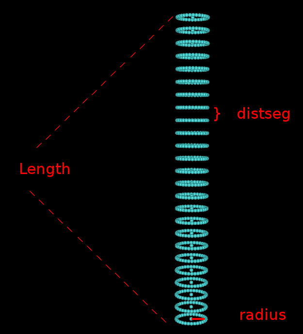
Most of the VolTrac
parameters shown in the video are intuitive, but for sake of
clarity we illustrate here the geometry of the template used in the
tracing:
3. Work flow for visualizing and manually editing the
traces
A frequently asked
question is how to visualize the VolTrac
traces in Sculptor. Here are four figures that show the procedure.
Click on the thumbnails to see the full size figures:
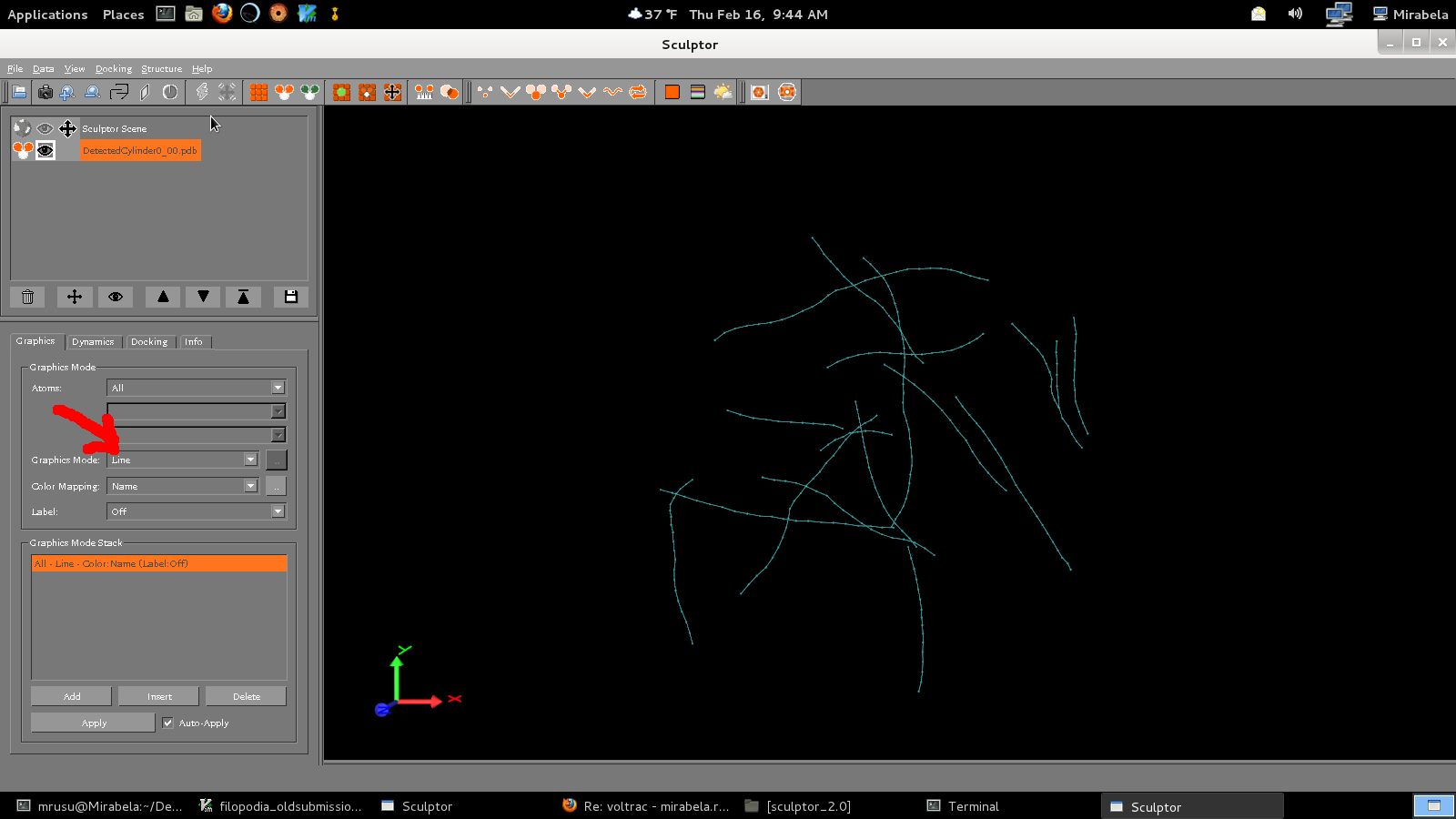
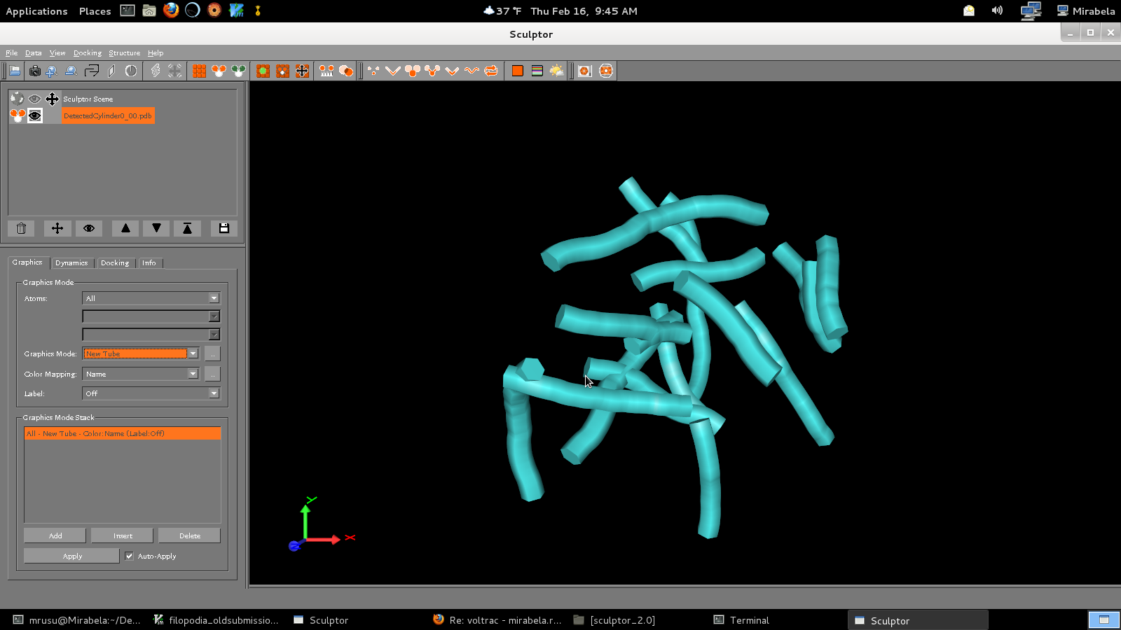
1. Load PDB
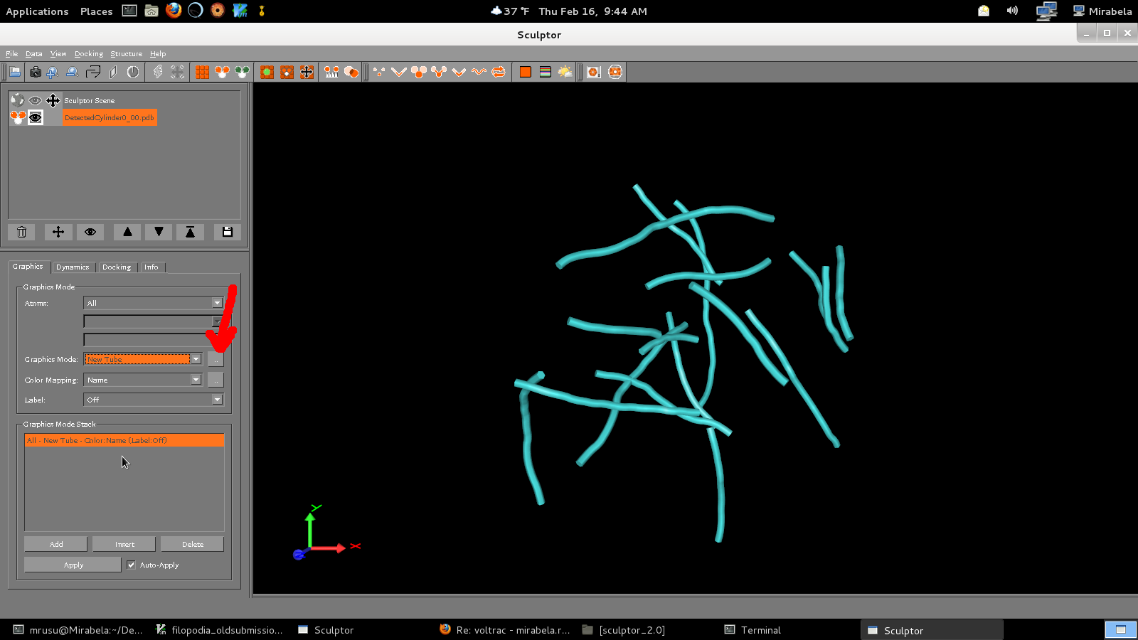
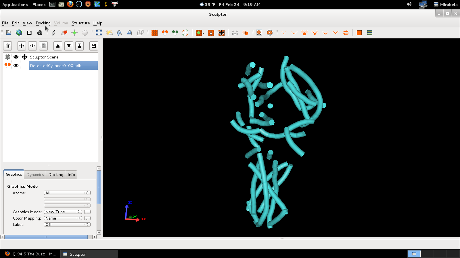
2. Show Tubes
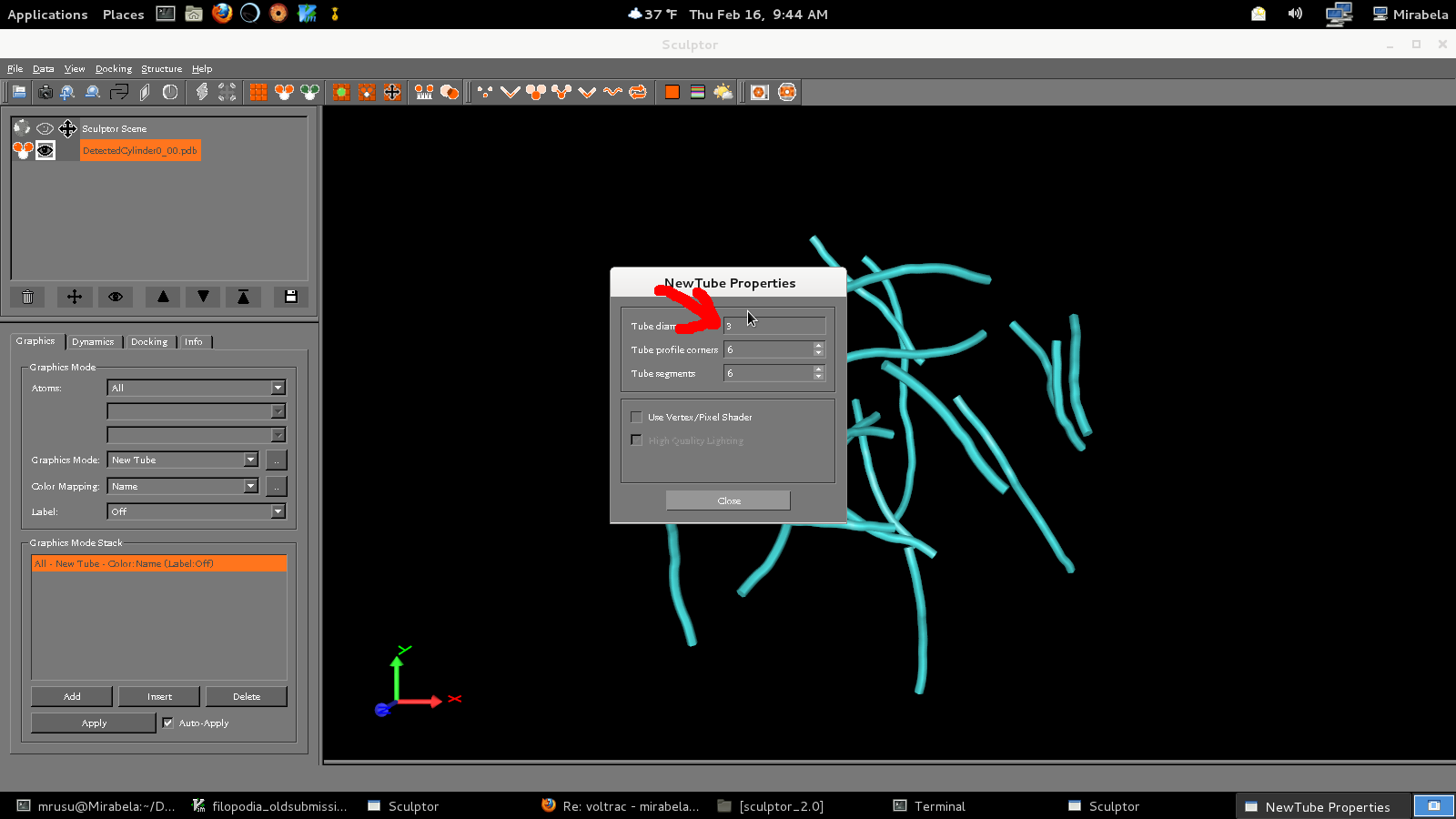
3. Increase Radius
4. Output
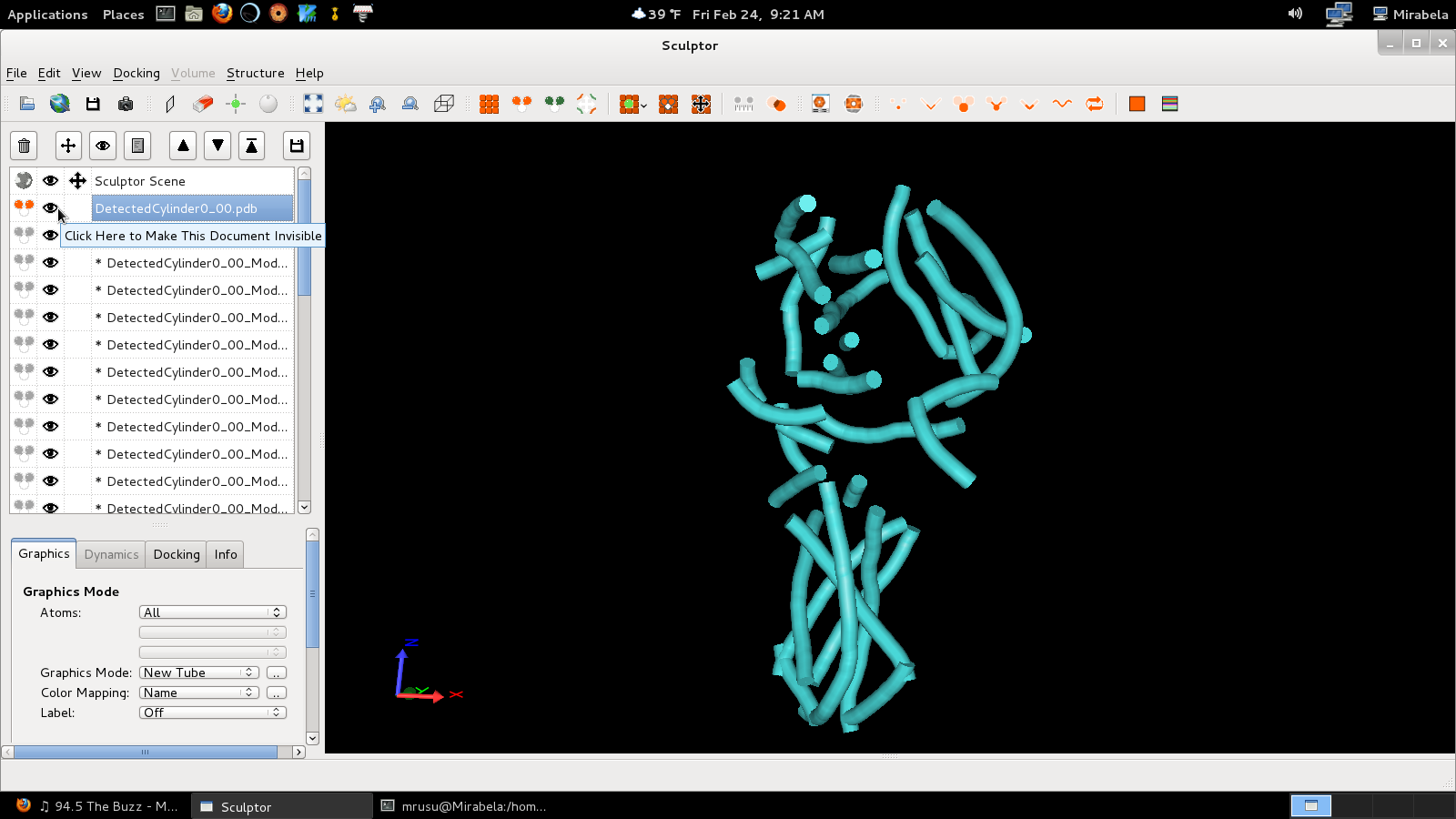
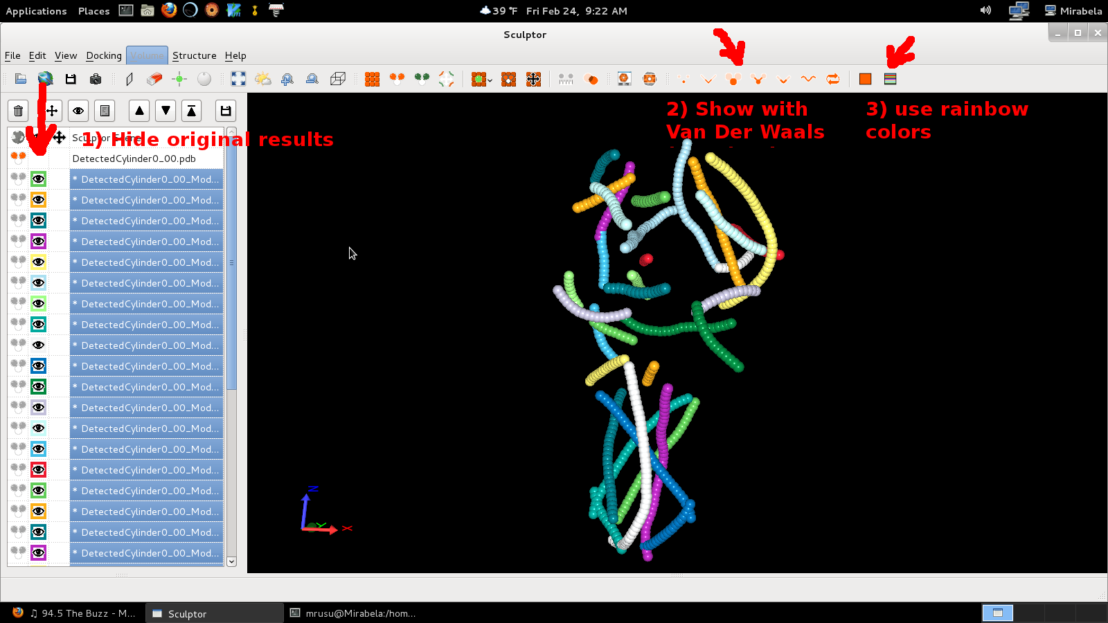
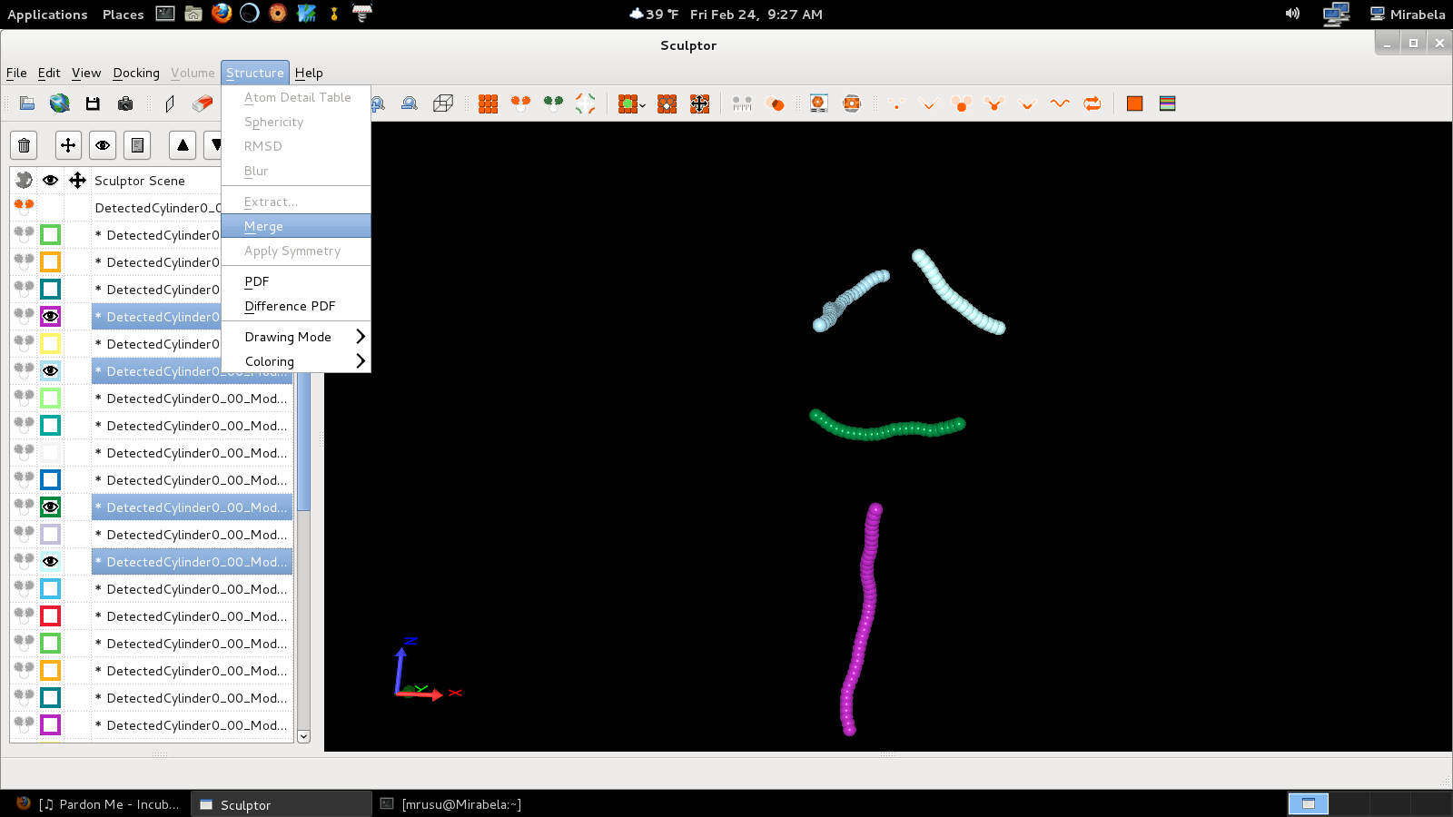
Often, a user may wish to manually edit the traces to eliminate false
positives (e.g. alpha helices placed in beta sheet regions). The manual
editing and merging of the results is described in the following series
of screenshots (click on the thumbnails to see the full size figures):
5. Show Tubes
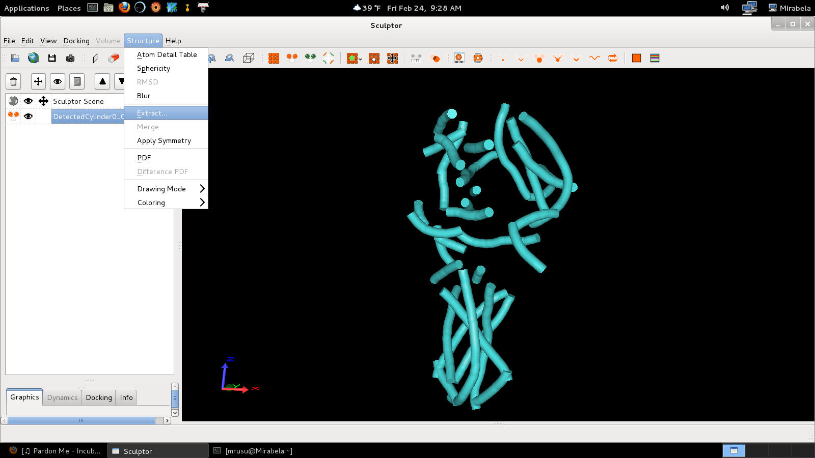
6. Select Extract
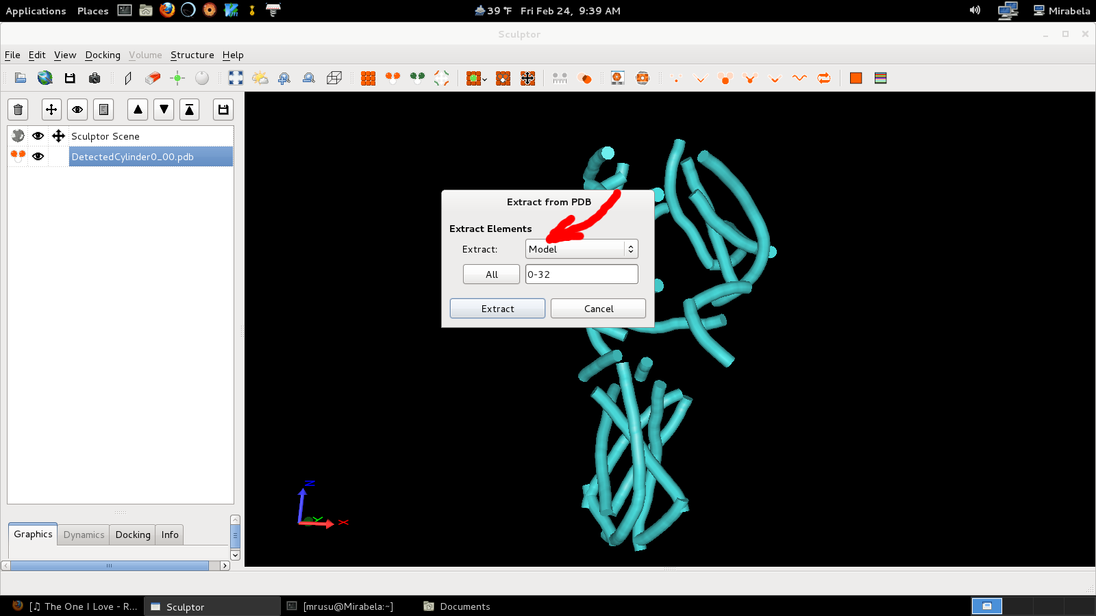
7. Extract Tubes
8. Hide Results
9. Change Rendering
10. Merge Highlighted
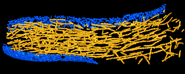
4. Work flow for tracing filaments in tomograms
If you are
interested in tracing filamentous density in 3D maps of
cellular structures from tomography or other in vivo imaging
techniques, we recommend to follow first the tutorials in steps 2 and 3
above to learn the basic functionality of the VolTrac algorithm.
Then, refer to Rusu
et al., 2012 which describes in the
main text the parameters and steps taken in the tracing of actin
filaments in a filopodium protrusion. Supplementary data files 2-6 of
this paper comprise snapshots of this workflow. Supplementary
data file 4 lists the steps taken prior to VolTrac, whereas
the VolTrac
parameters are given in the main text of the paper. The final results
shown in Fig. 3B of the paper are provided in supplementary file 6 for
comparison purposes. You can visualize these traces as described for
alpha-helices under step 3 above.